Lagrangian Mechanics and Principle of Least Action
I just watched a video from Veritasium about the history of the Principle of least action, and it was mind-blowing. As an engineer, I learned about Lagrangian mechanics in my undergraduate studies. I always use it as a tool to derive equations of motion, but I never fully understood the real meaning and connection behind it. After watching the video, I realized how beautiful the principle is and how it can be explained from the nature. I then started to dig deeper and decided to derive the Lagrangian equations of motion from the principle of least action myself.
Let’s start with the nature, we can observe that nature tends to follow some kind of path not arbitrarily, but in a unique way. For example, if we throw a ball into the air, it will follow a parabolic path. It will not follow any other path. Another example is the hanging chain, which will form a specific curve called a catenary. These exaples show that there is a unique path that nature follows, and this is the essence of the principle of least action.
From variational calculus, consider a functional $I$ that maps a function $y(x)$ to a real number, where $y(x)$ is a function of $x$ and $y^\prime(x)$ is its derivative as follows:
\[\begin{align} I[y] &= \int_{x_1}^{x_2} F\left(x, y(x), y^\prime(x)\right) dx \end{align}\]Consider a small perturbation of the function $y(x)$, such that $\bar{y}(x) = y(x) + \epsilon \eta(x)$, where $\eta(x)$ is a small perturbation function and $\epsilon$ is a magnitude of perturbation as illustrated in the figure below. Also, the perturbation $\eta(x)$ is zero at the boundaries, i.e., $\eta(x_1) = \eta(x_2) = 0$.
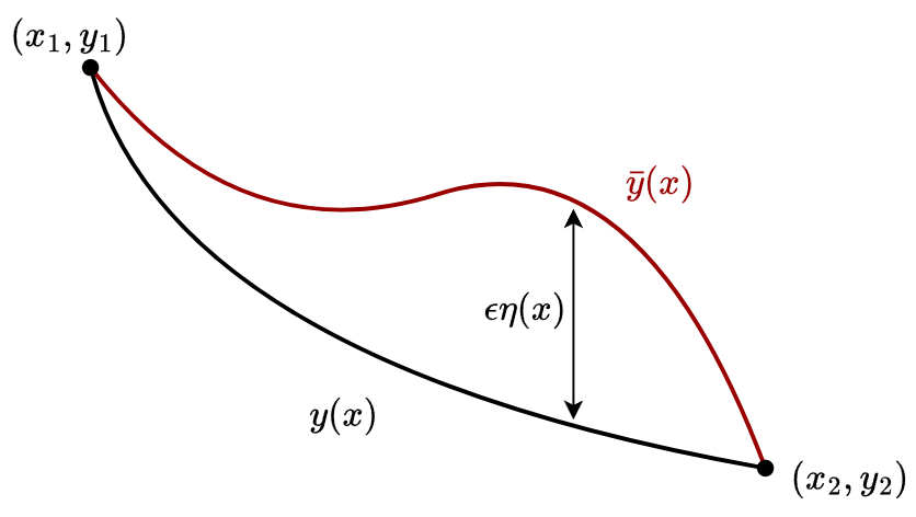 The original function $y(x)$ and the perturbed function $\bar{y}(x)$ with a small perturbation $\eta(x)$.
Suppose we want to find the function $y(x)$ that minimizes the functional $I[y]$. We can do this by considering the first variation of the functional at $\epsilon = 0$, where $\bar{y}(x)$ is equal to $y(x)$. The first variation of the functional is defined as:
\[\begin{align} \left. \frac{dI}{d\epsilon} \right|_{\epsilon=0} = 0 \label{eq:first_variation} \end{align}\]The functional becomes:
\[\begin{align*} \left. \frac{dI}{d\epsilon} \right|_{\epsilon=0} &= \left. \frac{d}{d\epsilon} \int_{x_1}^{x_2} F \left(x, \bar{y}(x), \bar{y}^\prime(x)\right) \right|_{\epsilon=0} dx \\ 0 &= \left. \int_{x_1}^{x_2} \frac{\partial}{\partial \epsilon} \left( F \left(x, \bar{y}(x), \bar{y}^\prime(x)\right) \right) \right|_{\epsilon=0} dx \tag*{(from Leibniz rule)} \\ &= \left. \int_{x_1}^{x_2} \left( \frac{\partial F}{\partial x} \frac{\partial x}{\partial \epsilon} + \frac{\partial F}{\partial \bar{y}}\frac{\partial \bar{y}}{\partial \epsilon} + \frac{\partial F}{\partial \bar{y}^\prime}\frac{\partial \bar{y}^\prime}{\partial \epsilon} \right) \right|_{\epsilon=0} dx \tag*{(from chain rule)} \\ &= \left. \int_{x_1}^{x_2} \left( \frac{\partial F}{\partial \bar{y}} \eta + \frac{\partial F}{\partial \bar{y}^\prime} \eta^\prime \right) \right|_{\epsilon=0} dx \end{align*}\]At $\epsilon = 0$ we have $\bar{y} = y$ and $\bar{y}^\prime = y^\prime$, so we can rewrite the equation as:
\[\begin{align*} 0 &= \int_{x_1}^{x_2} \left( \frac{\partial F}{\partial y} \eta + \frac{\partial F}{\partial y^\prime} \eta^\prime \right) dx \end{align*}\]From integration by parts, $\int u \, dv = uv - \int v \, du$, where:
\[u = \frac{\partial F}{\partial y^\prime}, \quad du = \frac{d}{dx} \left( \frac{\partial F}{\partial y^\prime} \right) dx , \quad dv = \eta^\prime dx, \quad v = \eta\]So we can rewrite the second term as follows:
\[\begin{align*} \int_{x_1}^{x_2} \frac{\partial F}{\partial y^\prime} \eta^\prime dx &= \left . \frac{\partial F}{\partial y^\prime} \eta \right|_{x_1}^{x_2} - \int_{x_1}^{x_2} \frac{d}{dx} \left( \frac{\partial F}{\partial y^\prime} \right) \eta dx \\ &= - \int_{x_1}^{x_2} \frac{d}{dx} \left( \frac{\partial F}{\partial y^\prime} \right) \eta dx \tag*{(since $\eta(x_1) = \eta(x_2) = 0$)} \end{align*}\]Now we can substitute this back into the original equation:
\[\begin{align*} 0 &= \int_{x_1}^{x_2} \left( \frac{\partial F}{\partial y} \eta - \frac{d}{dx} \left( \frac{\partial F}{\partial y^\prime} \right) \eta \right) dx \\ &= \int_{x_1}^{x_2} \left( \frac{\partial F}{\partial y} - \frac{d}{dx} \left( \frac{\partial F}{\partial y^\prime} \right) \right) \eta dx \end{align*}\]Since $\eta(x)$ is arbitrary, the only way for the integral to be zero for all $\eta(x)$ is if the term $\frac{\partial F}{\partial y} - \frac{d}{dx} \left( \frac{\partial F}{\partial y^\prime} \right)$ is zero. So we have:
\[\begin{align*} \frac{\partial F}{\partial y} - \frac{d}{dx} \left( \frac{\partial F}{\partial y^\prime} \right) = 0 \end{align*}\]Let $F = L(x, y, y^\prime)$, where $L$ is the Lagrangian function, $y$ is the generalized coordinate $q$, $y^\prime$ becomes the generalized velocity $\dot{q}$, and $x$ is time $t$. Then, we get the famous Euler-Lagrange equation:
\[\begin{align*} \frac{\partial L}{\partial q} - \frac{d}{dt} \left( \frac{\partial L}{\partial \dot{q}} \right) = 0 \end{align*}\]Also, we can define the action $S$ as the integral of the Lagrangian over time:
\[\begin{align*} S[q] &= \int_{t_1}^{t_2} L(t, q, \dot{q}) dt \end{align*}\]Then the Principle of Least Action states that the path taken by the system is the one that minimizes the action similar to Eq. \ref{eq:first_variation}, i.e.,
\[\begin{align*} \delta S[q] &= 0 \end{align*}\]This equation may look weird at first, but we can interpret it by considering the Lagrangian is the difference between the kinetic energy $T = \frac{1}{2}m\dot{q}^2$ and potential energy $V$ of the system, i.e., $L = T - V$. Then, we have:
\[\begin{align*} \frac{\partial L}{\partial q} &= -\frac{\partial V}{\partial q} \\ \frac{d}{dt} \left( \frac{\partial L}{\partial \dot{q}} \right) &= m\ddot{q} \end{align*}\]Then, the Euler-Lagrange equation becomes:
\[\begin{align*} -\frac{\partial V}{\partial q} - m\ddot{q} &= 0 \\ - \frac{\partial V}{\partial q} &= m\ddot{q} \\ F &= m\ddot{q} \end{align*}\]Voilà! We get the famous Newton’s second law of motion, $F = ma$. So, in the end, these two equations are the same, and the Euler-Lagrange equation is just a more general form of Newton’s second law (see more explaination at Deriving the Euler-Lagrange Equation). We can also extend the Euler-Lagrange equation to systems with external forces as follows:
\[\begin{align*} \frac{d}{dt} \left( \frac{\partial L}{\partial \dot{q}} \right) - \frac{\partial L}{\partial q} = F_{\text{ext}} \end{align*}\]I prefer to write it this way because it is more convenient to use with the sign convention of the force $F_{\text{ext}}$ as the same direction with the generalized coordinate $q$.
Extra: Leibniz rule
We want to show the Leibniz rule (see more explaination at Leibniz Rule), which states that:
We can derive it as follows:
\[\begin{align*} \frac{d}{dx} \int_{a}^{b} f(x, y) dy = \lim\limits_{\Delta x \to 0} \frac{1}{\Delta x} \left( \int_{a}^{b} f(x + \Delta x, y) dy - \int_{a}^{b} f(x, y) dy \right) \\ \end{align*}\]Consider the Taylor expansion of $f(x + \Delta x, y)$ around $x$:
\[\begin{align*} f(x + \Delta x, y) &= f(x, y) + \frac{\partial f}{\partial x} \Delta x + \mathcal{O}(\Delta x^2) \end{align*}\]Substituting this into the integral gives:
\[\begin{align*} \frac{d}{dx} \int_{a}^{b} f(x, y) dy &= \lim\limits_{\Delta x \to 0} \frac{1}{\Delta x} \left( \int_{a}^{b} f(x, y) + \left( \frac{\partial f}{\partial x} \Delta x + \mathcal{O}(\Delta x^2) \right) dy - \int_{a}^{b} f(x, y) dy \right) \\ &= \lim\limits_{\Delta x \to 0} \left( \int_{a}^{b} \left( \frac{\partial f}{\partial x} + \mathcal{O}(\Delta x) \right) dy \right) \\ &= \int_{a}^{b} \left( \frac{\partial f}{\partial x} \right) dy \end{align*}\]